COVID-19 spread predictor
- 7 mins
Prediction for the spread of COVID-19 using Epidemiological Models
SUMMARY
I developed a model to predict the curves of contamination, deaths and recoveries in the cases of COVID-19. Unlike time series analyzes, the model uses regression techniques to predict the rates of change as a function of the current number of contaminations, deaths and recoveries over time. With this, I hope that the model will be able to learn how the time derivatives change as we observe variations (even sudden ones) in the numbers of cases and, after a numerical integration, be able to predict future data with greater precision than simple temporal projection with regressors in time series analysis techniques.
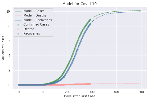
Table of Contents
1. Description
1.1 Epidemiological Models
The reader familiar with epidemiological models, can go to section 1.2.
The simplest epidemiological models used for modeling SARS-COVID-19 are based on first principles and defined in terms of differential equations on quantities that describe the epidemiological status of the population. In the simplest cases, these quantities are:
- D(t): cumulative number of deaths on time t;
- C(t): cumulative number of confirmed cases on time t;
- R(t): cumulative number of recovered cases on time t;
- I(t): current number infections on time t
Fixing the number of people constant, only three of these four functions are independent, and, in general, the function C(t) is eliminated by the relation C (t) = I (t) + R (t ) + D (t) .
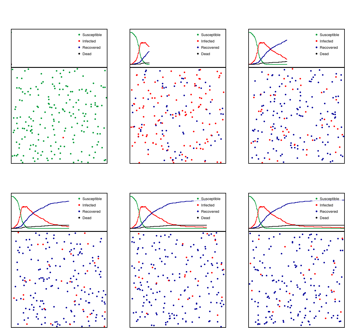
An additional concept that appears in the models is that of susceptibility and takes into account that the entire population cannot, in fact, be subject to infection. It is to be expected that the number of susceptible people will be a dynamic variable, since cases of reinfection are practically non-existent (or certainly very unlikely in relation to cases of first infection). This variable is called:
- S(t): number of individuals susceptible to infection over time t
Susceptible people, when infected, leave the group of S(t) and become C(t). As a consequence:
Intuitively, the rate of infection is correlated with the number of susceptible people and the number of people actively infected. A simple model of this relationship is:
which, through equation (1), naturally leads to:
where k_s > 0.
Another expected behavior is that both the rate of people recovered and the rate of deaths are proportional in a given time t to the number of people actively infected:
e
where k_r,k_d > 0.
Alternatively, you can use the link C(t) = I (t) + R (t) + D (t) to deduct the differential equation for I (t) :
The model described above is well founded, but takes several hypotheses into account. It has been successfully applied to describe the evolution of Covid-19 in different regions. However, these hypotheses are associated with idealized cases and, because of this, the model is not general enough to adapt to the modeling of Covid-19 cases. When this occurs, the authors call for generalizations of the models, generally based on different equations of the type:
where the algebraic functions f_s , f_i , f_d and f_r are determined according to the problem under study.
In my opinion, the biggest problem with the application of epidemiological models to Covid-19 modeling is in the human factor. Several times, pathological behaviors were observed in the curves of Covid-19 (as in the case of China and the USA), which are abrupt or even mild changes, but which do not respect the equations in the model. What is wrong in this case is, in general, due to human action. Whether by changing collective behavior (collective abandonment of isolation rules), political influence on social behavior, changes in public policy rules, etc. In such cases, Machine Learning models can be used.
[1] Ranjan, R. (2020). Predictions for COVID-19 outbreak in India using Epidemiological models. medRxiv.
[2] Hethcote, H. W. (2009). The basic epidemiology models: models, expressions for R0, parameter estimation, and applications. In Mathematical understanding of infectious disease dynamics (pp. 1-61).
<h2>1.2 Machine Learning Models</h2>
Unlike epidemiological models, machine learning models are, in general, structured in a different way. There is a wide range of approaches, but the dynamic variables C (t) , D (t) , R (t) and I (t) are generally taken as time series. As this approach is data oriented, there is no reference to the dynamic variable S (t) , since it carries an abstract notion (that of the number of susceptible people) that is something inaccessible. This type of approach, in the short term, is quite satisfactory because it allows forecasts of the evolution of the disease in the coming days. However, in the long run, predictions are more dispersed and inaccurate. The reason for this is that the learning models with this characteristic relate each of the dynamic variables only with time. However, as discussed in the topic of epidemiological models, there are correlations between the variables C (t) , D (t) , R (t) and I (t) .
The model proposed here is described as follows: I want to obtain a set of different equations similar to that of Eqs. (5), however, considering C (t) instead of I (t) .
- Since it is not possible to accurately infer a time series for S (t) , this variable won’t be considered.
- In addition, I want to allow f functions to depend directly on time to.
In these considerations, the system will be reduced to:
-
The f functions will be determined by applying regression models. With this, I will obtain three models of machine learning capable of predicting the variation rates of C , D and R receiving data from t_ {in} , C (t_ {in}) , D (t_ {in}) and R (t_ {in}) as input.
-
With the variation rates model, I can integrate the model in the opposite direction, taking the last data as an initial condition. In this process, the machine learning model will be validated
-
As the model validated, future predictions can be performed
2. Python Package
Dependencies
You need Python 3.7 or later to use cov19. You can find it at python.org. You also need setuptools, pandas, pygtc and tqdm packages, which is available from PyPI. If you have pip, just run:
pip install pandas
pip install pygtc
pip install setuptools
pip install tqdm
Installation
You can install the package via PyPI:
pip install cov19
Alternatively, you can clone this repo to your local machine using:
git clone https://github.com/emdemor/cov19
3. Features
- Support for different epidemiological models
- Monte Carlo Markov Chains (MCMC) approach to fit patameters
- Data from multiple trusted and reliable sources compiled by Microsoft and accessible in www.bing.com/covid.
4. Results
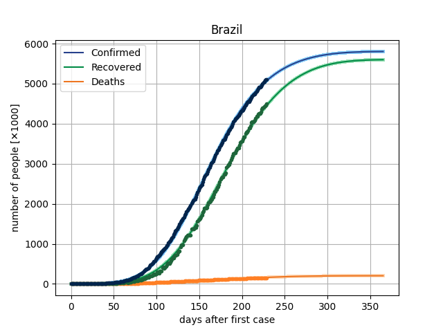
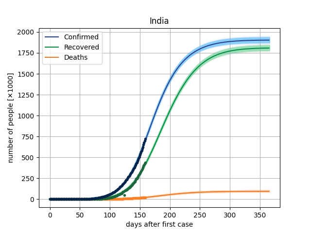
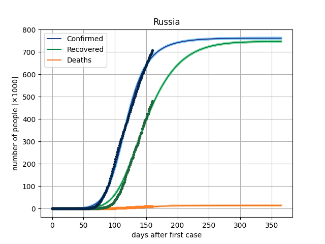
The main result in this version is to plot de curves from the model for a specific parameter vector and compare this with dataset. In covid/stat.py, functions has been implemented to generate an MCMC sample, through which it will be possible to make inferences of the parametric intervals.
5. Dataset
Here, we are using the Microsoft Data, from the repo https://github.com/microsoft/Bing-COVID-19-Data. ]
